
I’m pleased to announce a new release of Kojo. The following are the highlights since the last announcement:
1. Upgrade to Java 11 and Scala 2.13.2
This release includes updates to the core foundational technologies within Kojo:
- The Java runtime (JVM) has been upgraded from version 8 to version 11 — for access to the latest stable JVM technology. The upgrade to Java 11 also provided an opportunity to trim the size of the JVM that is bundled with Kojo (by removing unused components like JavaFX). This has resulted in a decrease of around 25% in the size of the Kojo installer.
- Scala has been upgraded to 2.13.2 (from 2.12.10). This provides improvements to the collections framework and overall performance, in addition to other internal improvements.
2. Generative art enhancements
2(a) Neural style transfer using deep learning
Neural style transfer (NST) is a deep-learning technique that lets you apply the style of one image to the content of another image.
Kojo now supports NST via its easy to use picture transformation syntax. Using this syntax, applying one or more styles (from one or more images) to a pattern is as simple as doing:
val pic = effect(style1) * effect(style2) -> pattern
draw(pic)
Here is an example drawing made in Kojo using NST:

This feature is based on PyTorch. To use NST in Kojo, you need to set up a Python virtual environment with PyTorch, and then do a bit more. So setting this up is a little bit of work for now. But once things are set up, this feature is easy to use (as described above).
2(b) Immediate mode canvas graphics based on a Processing like API
For scenarios (like agent-motion based generative art) where you need to draw hundreds of thousands of objects on the screen, Kojo now includes an immediate mode API — modelled on the Processing API. To use this API, you need to do the following:
- Create an instance of a class (called Sketch by convention) that has two methods —
setup()anddrawLoop(). - Give this instance to the
canvasSketch(sketch)command. - After this, your
setup()code will be called once and yourdrawLoop()code will be called at 50 FPS.
Within setup() and drawLoop() you can use the Processing like API.
To make it easy to get going with an immediate mode sketch, Kojo includes a code template for this. Just type in canvasSk in the script editor and press Ctrl+Alt+Space. Then select the canvasSketch template from the code-completion window that pops up. That will give you the following ready to run code:
cleari()
originBottomLeft()
setBackground(white)

class Sketch {
var x = 0
  def setup(surface: CanvasDraw) {
    import surface._
    strokeWeight(4)
    rect(0, cheight/2, 40, 40)
  }

  def drawLoop(surface: CanvasDraw) {
    import surface._
    background(255)
    x += 2
    rect(x, cheight/2, 40, 40)
  }
}

val sketch = new Sketch
canvasSketch(sketch)
Now tweak this as desired. Within setup() and drawLoop(), you can can use code completion on the surface object to see what (Processing like) drawing commands are available to you.
Here is a larger example that uses this API :

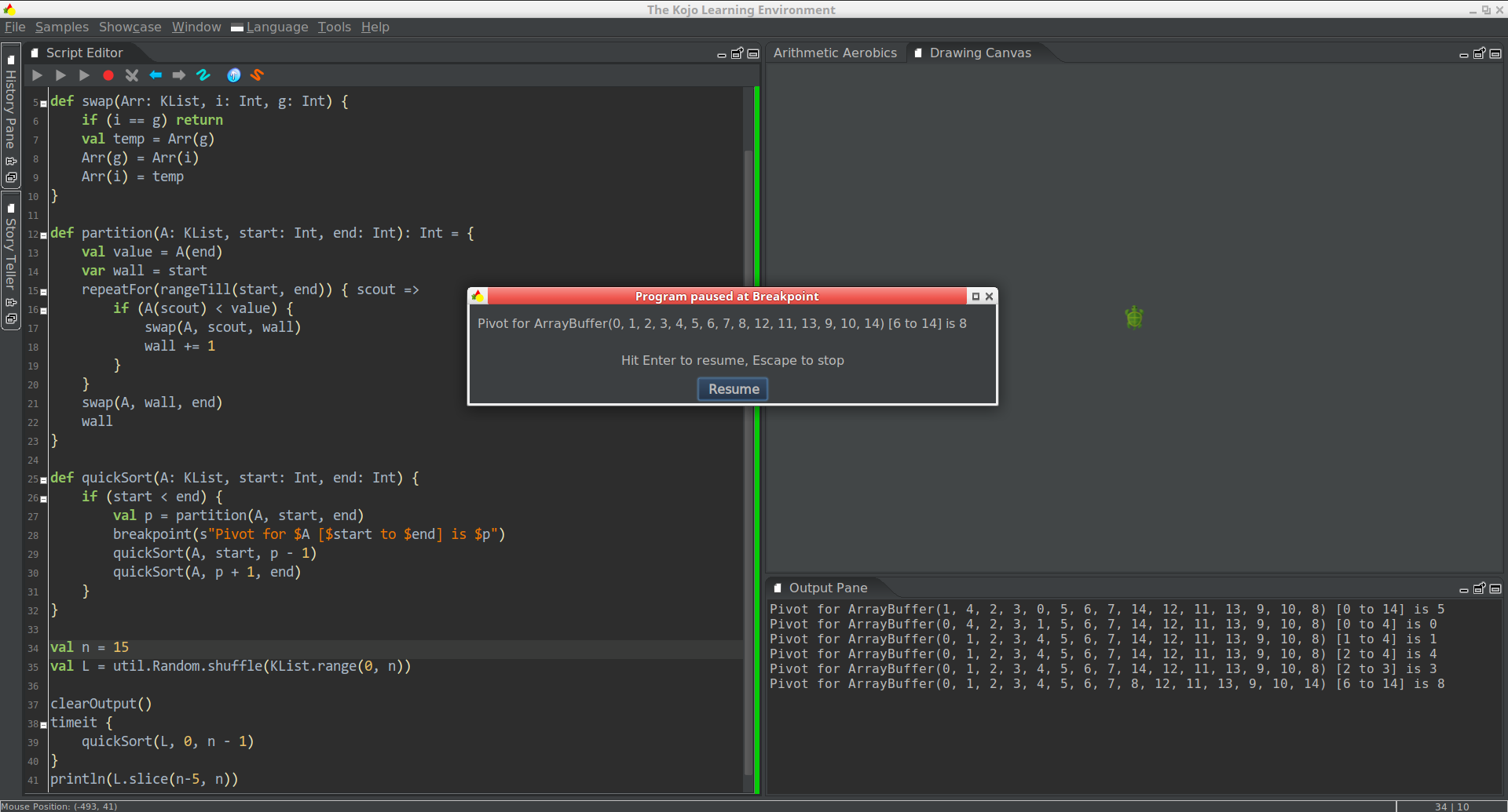
3. Breakpoint command
Kojo now includes a breakpoint command which makes it easy to debug/understand programs. You can put breakpoint(someData) on any line in a program, and when the program runs it will stop at that line and show you the value of someData. someData can be a formatted string, so you can put in whatever descriptive string you want to see — to help you to debug/understand the program. All the provided data across successive breakpoint calls is also printed in the output pane, so the output there gives you a nice view of how the data of interest in your program is evolving as the program runs.
This feature is especially useful in debugging/understanding two kinds of scenarios:
- Graphical drawing — for example when you draw a grid, you can put a
breakpointin your grid-cell drawing code, and then see the grid being drawn cell by cell, along with the desired data for each cell. - Algorithms — you can put a
breakpointat the input/output to a function to see, step by step, exactly what comes in to, and goes out of, the function. You can see similar information with tracing, but with abreakpointyou can stop a program at a point of interest, look at the data values there, and then proceed step by step.
Here are screenshots of both of the above scenarios:

4. New tutorials and book
New tutorials and a beginner-level book in lesson-plan format are now available on the Tutorials page on the Kojo Docs website. Here are a few examples (ranging from the simple to the not so simple) of the kinds of drawings you can make with the help of the tutorials:


5. Other enhancements
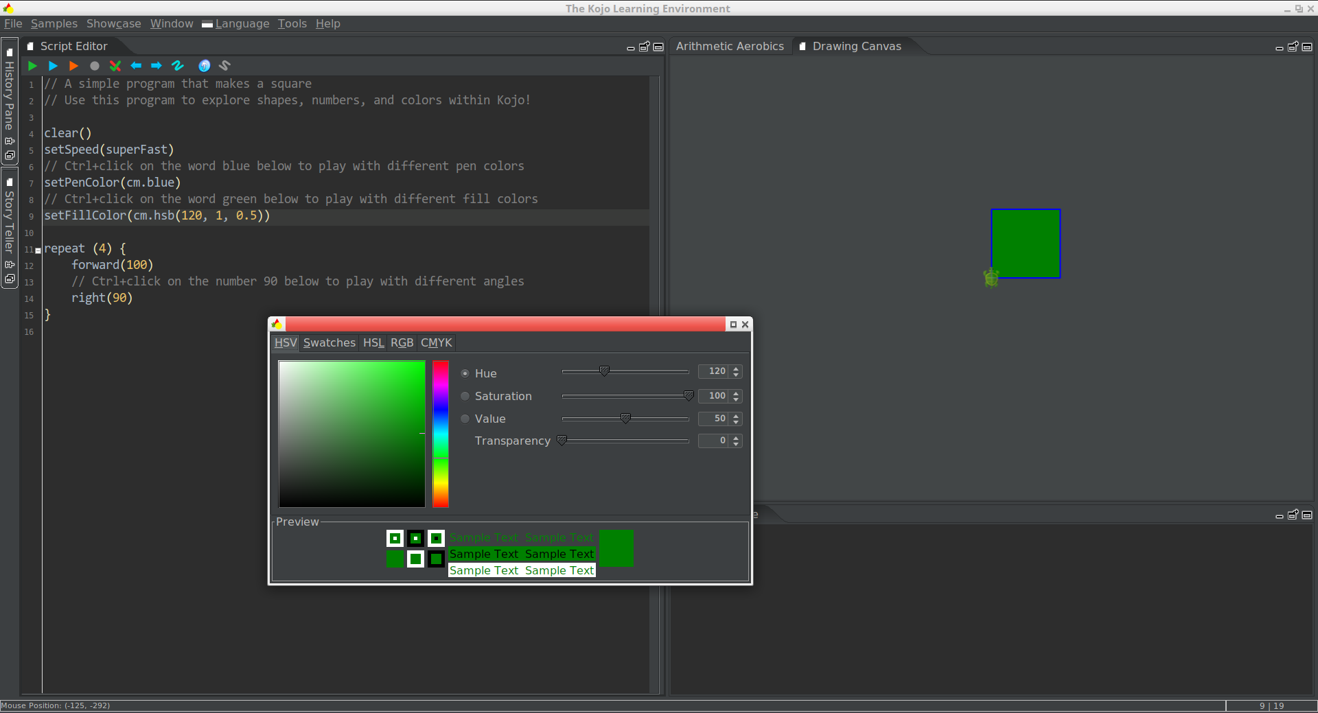
5(a) Support for HSB colors in the ColorMaker
The ColorMaker now supports the HSB/HSV color model, in addition to the HSL and RGB models. This is fully integrated with IPM (Interactive Program Manipulation), so you can Ctrl+Click on any HSB color in your code to bring up the color-tweaker window:
For quick reference, the following are some of the ColorMaker functions for creating colors (here shown creating a green or a half-transparent green color):
// cm is an abbreviation for ColorMaker
cm.rgb(0, 255, 0)
cm.rgba(0, 255, 0, 127)
cm.hsl(120, 1.0, 0.5)
cm.hsla(120, 1.0, 0.5, 0.5)
cm.hsl(120, 1.0, 1.0)
cm.hsla(120, 1.0, 1.0, 0.5)
cm.hex(0x00ff00)
cm.hex(0x7f00ff00)
You can also create gradients and textures via the following ColorMaker functions:
// use code completion to fill out the args
cm.linearGradient
cm.linearMultipleGradient
cm.radialGradient
cm.radialMultipleGradient
cm.texture
5(b) timeit command
A new timeit command makes it easy to time your code. For example:
// type KList = ArrayBuffer[Int]
val n = 1500000
val L = util.Random.shuffle(KList.range(0, n))

clearOutput()
timeit {
  quickSort(L)
}
println(L.slice(n - 5, n))
The above prints out the following in the output pane:
Timed code took 3.039 seconds
ArrayBuffer(1499995, 1499996, 1499997, 1499998, 1499999)
That’s it for now.
As always, the new version of Kojo is available from the Kojo Download Page. If you run into any difficulties, let us know.
Enjoy!

